I’d like to share the results of the quick benchmark tests I’ve done to measure the performance of the R-tree implementation included in the mdds library since 1.4.0.
Brief overview on R-tree
R-tree is a data structure designed for optimal query performance on spatial data. It is especially well suited when you need to store a large number of spatial objects in a single store and need to perform point- or range-based queries. The version of R-tree implemented in mdds is a variant known as R*-tree, which differs from the original R-tree in that it occasionally forces re-insertion of stored objects when inserting a new object would cause the target node to exceed its capacity. The original R-tree would simply split the node unconditionally in such cases. The reason behind R*-tree’s choice of re-insertion is that re-insertion would result in the tree being more balanced than simply splitting the node without re-insertion. The downside of such re-insertion is that it would severely affect the worst case performance of object insertion; however, it is claimed that in most real world use cases, the worst case performance would rarely be hit.
That being said, the insertion performance of R-tree is still not very optimal especially when you need to insert a large number of objects up-front, and unfortunately this is a very common scenario in many applications. To mitigate this, the mdds implementation includes a bulk loader that is suitable for mass-insertion of objects at tree initialization time.
What is measured in this benchmark
What I measured in this benchmark are the following:
- bulk-loading of objects at tree initialization,
- the size() method call, and
- the average query performance.
I have written a specially-crafted benchmark program to measure these three categories, and you can find its source code here. The size() method is included here because in a way it represents the worst case query scenario since what it does is visit every single leaf node in the entire tree and count the number of stored objects.
The mdds implementation of R-tree supports arbitrary dimension sizes, but in this test, the dimension size was set to 2, for storing 2-dimensional objects.
Benchmark test design
Here is how I designed my benchmark tests.
First, I decided to use map data which I obtained from OpenStreetMap (OSM) for regions large enough to contain the number of objects in the millions. Since OSM does not allow you to specify a very large export region from its web interface, I went to the Geofabrik download server to download the region data. For this benchmark test, I used the region data for North Carolina, California, and Japan’s Chubu region. The latitude and longitude were used as the dimensions for the objects.
All data were in the OSM XML format, and I used the XML parser from the orcus project to parse the input data and build the input objects.
Since the map objects are not necessarily of rectangular shape, and not necessarily perfectly aligned with the latitude and longitude axes, the test program would compute the bounding box for each map object that is aligned with both axes before inserting it into R-tree.
To prevent the XML parsing portion of the test to affect the measurement of the bulk loading performance, the map object data gathered from the input XML file were first stored in a temporary store, and then bulk-loaded into R-tree afterward.
To measure the query performance, the region was evenly split into 40 x 40 sub-regions, and a point query was performed at each point of intersection that neighbors 4 sub-regions. Put it another way, a total of 1521 queries were performed at equally-spaced intervals throughout the region, and the average query time was calculated.
Note that what I refer to as a point query here is a type of query that retrieves all stored objects that intersects with a specified point. R-tree also allows you to perform area queries where you specify a 2D area and retrieve all objects that overlap with the area. But in this benchmark testing, only point queries were performed.
For each region data, I ran the tests five times and calculated the average value for each test category.
It is worth mentioning that the machine I used to run the benchmark tests is a 7-year old desktop machine with Intel Xeon E5630, with 4 cores and 8 native threads running Ubuntu LTS 1804. It is definitely not the fastest machine by today’s standard. You may want to keep this in mind when reviewing the benchmark results.
Benchmark results
Without further ado, these are the actual numbers from my benchmark tests.
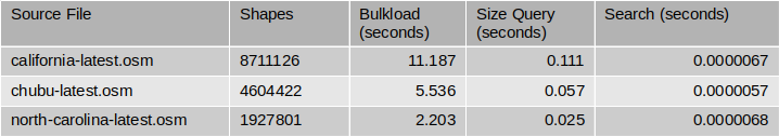
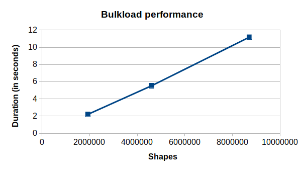
The Shapes column shows the numbers of map objects included in the source region data. When comparing the number of shapes against the bulk-loading times, you can see that the bulk-loading time scales almost linearly with the number of shapes:
You can also see a similar trend in the size query time against the number of shapes:

The point query search performance, on the other hand, does not appear to show any correlation with the number of shapes in the tree:
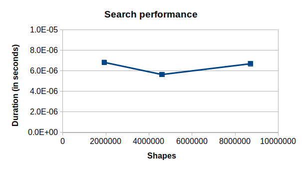
This makes sense since the structure of R-tree allows you to only search in the area of interest regardless of how many shapes are stored in the entire tree. I’m also pleasantly surprised with the speed of the query; each query only takes 5-6 microseconds on this outdated machine!
Conclusion
I must say that I am overall very pleased with the performance of R-tree. I can already envision various use cases where R-tree will be immensely useful. One area I’m particularly interested in is spreadsheet application’s formula dependency tracking mechanism which involves tracing through chained dependency targets to broadcast cell value changes. Since the spreadsheet organizes its data in terms of row and column positions which is 2-dimensional, and many queries it performs can be considered spatial in nature, R-tree can potentially be useful for speeding things up in many areas of the application.