Benchmark results on mdds multi_type_vector

In this post, I’m going to share the results of some benchmark testing I have done on multi_type_vector, which is included in the mdds library. The benchmark was done to measure the impact of the change I made recently to improve the performance on block searches, which will affect a major part of its functionality.

Background

One of the data structures included in mdds, called multi_type_vector, stores values of different types in a single logical vector. LibreOffice Calc is one primary user of this. Calc uses this structure as its cell value store, and each instance of this value store represents a single column instance.

Internally, multi_type_vector creates multiple element blocks which are in turn stored in its parent array (primary array) as block structures. This primary array maps a logical position of a value to the actual block structure that stores it. Up to version 1.5.0, this mapping process involved a linear search that always starts from the first block of the primary array. This was because each block structure, though it stores the size of the element block, does not store its logical position. So the only way to find the right element block that intersects the logical position of a value is to scan from the first block and keep accumulating the sizes of the encountered blocks. The following diagram depicts the structure of multi_type_vector’s internal store as of 1.5.0:

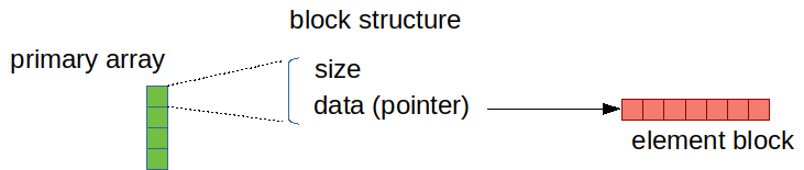
The reason for not storing the logical positions of the blocks was to avoid having to update them after shifting the blocks after value insertion, which is quite common when editing spreadsheet documents.

Of course, sometimes one has to perform repeated searches to access a number of element values across a number of element blocks, in which case, always starting the search from the first block, or block 0, in every single search can be prohibitively expensive, especially when the vector is heavily fragmented.

To alleviate this, multi_type_vector provides the concept of position hints, which allows the caller to start the search from block N where N > 0. Most of multi_type_vector’s methods return a position hint which can be used for the next search operation. A position hint object stores the last position of the block that was either accessed or modified by the call. This allows the caller to chain all necessary search operations in such a way to scan the primary array no more than once for the entire sequence of search operations. It was largely inspired by std::map’s insert method which provides a very similar mechanism. The only prerequisite is that access to the elements occur in perfect ascending order. For the most part, this approach worked quite well.

The downside of this is that there are times you need to access multiple element positions and you cannot always arrange your access pattern to take advantage of the position hints. This is the case especially during multi-threaded formula cell execution routine, which Calc introduced some versions ago. This has motivated us to switch to an alternative lookup algorithm, and binary search was the obvious replacement.

Binary search

Binary search is an algorithm well suited to find a target value in an array where the values are stored in sorted order. Compared to linear search, binary search performs much faster except for very small arrays. People often confuse this with binary search tree, but binary search as an algorithm does not limit its applicability to just tree structure; it can be used on arrays as well, as long as the stored values are sorted.

While it’s not very hard to implement binary search manually, the C++ standard library already provides several binary search implementations such as std::lower_bound and std::upper_bound.

Switch from linear search to binary search

The challenge for switching from linear search to binary search was to refactor multi_type_vector’s implementation to store the logical positions of the element blocks and update them real-time, as the vector gets modified. The good news is that, as of this writing, all necessary changes have been done, and the current master branch fully implements binary-search-based block position lookup in all of its operations.

Benchmarks

To get a better idea on how this change will affect the performance profile of multi_type_vector, I ran some benchmarks, using both mdds version 1.5.0 – the latest stable release that still uses linear search, and mdds version 1.5.99 – the current development branch which will eventually become the stable 1.6.0 release. The benchmark tested the following three scenarios:

  1. set() that modifies the block layout of the primary array. This test sets a new value to an empty vector at positions that monotonically increase by 2, until it reaches the end of the vector.
  2. set() that updates the value of the last logical element of the vector. The update happens without modifying the block layout of the primary array. Like the first test, this one also measures the performance of the block position lookup, but since the block count does not change, it is expected that the block position lookup comprises the bulk of its operation.
  3. insert() that inserts a new element block at the logical mid-point of the vector and shifts all the elements that occur below the point of insertion. The primary array of the vector is made to be already heavily fragmented prior to the insertion. This test involves both block position lookup as well as shifting of the element blocks. Since the new multi_type_vector implementation will update the positions of element blocks whose logical positions have changed, this test is designed to measure the cost of this extra operation that was previously not performed as in 1.5.0.

In each of these scenarios, the code executed the target method N number of times where N was specified to be 10,000, 50,000, or 100,000. Each test was run twice, once with position hints and once without them. Each individual run was then repeated five times and the average duration was computed. In this post, I will only include the results for N = 100,000 in the interest of space.

All binaries used in this benchmark were built with a release configuration i.e. on Linux, gcc with -O3 -DNDEBUG flags was used to build the binaries, and on Windows, MSVC (Visual Studio 2017) with /MD /O2 /Ob2 /DNDEBUG flags was used.

All of the source code used in this benchmark is available in the mdds perf-test repository hosted on GitLab.

The benchmarks were performed on machines running either Linux (Ubuntu LTS 1804) or Windows with a variety of CPU’s with varying number of native threads. The following table summarizes all test environments used in this benchmark:

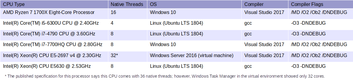
It is very important to note that, because of the disparity in OS environments, compilers and compiler flags, one should NOT compare the absolute values of the timing data to draw any conclusions about CPU’s relative performance with each other.

Results

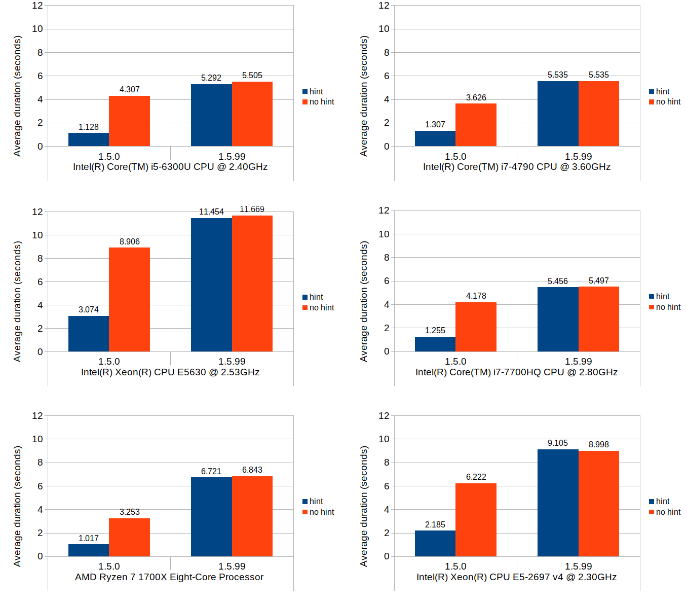
Scenario 1: set value at monotonically increasing positions

This scenario tests a set of operations that consists of first seeking the position of a block that intersects with the logical position, then setting a new value to that block which causes that block to split and a new value block inserted at the point of split. The test repeats this process 100,000 times, and in each iteration the block search distance progressively increases as the total number of blocks increases. In Calc’s context, scenarios like this are very common especially during file load.

Without further ado, here are the results:

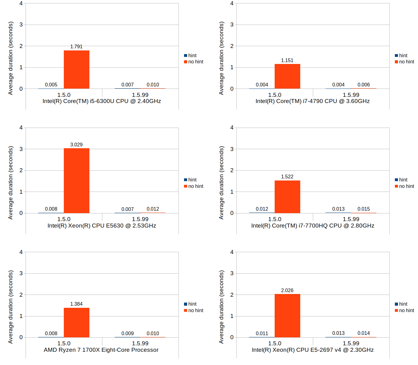
You can easily see that the binary search (1.5.99) achieves nearly the same performance as the linear search with position hints in 1.5.0. Although not very visible in these figures due to the scale of the y-axes, position hints are still beneficial and do provide small but consistent timing reduction in 1.5.99.

Scenario 2: set at last position

The nature of what this scenario tests is very similar to that of the previous scenario, but the cost of the block position lookup is much more emphasized while the cost of the block creation is eliminated. Although the average durations in 1.5.0 without position hints are consistently higher than their equivalent values from the previous scenario across all environments, the overall trends do remain similar.

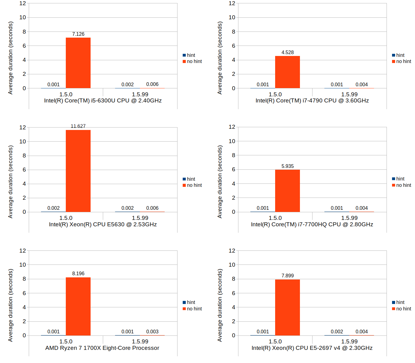
Scenario 3: insert and shift

This last scenario was included primarily to test the cost of updating the stored block positions after the blocks get shifted, as well as to quantify how much increase this overhead would cause relative to 1.5.0. In terms of Calc use case, this operation roughly corresponds with inserting new rows and shifting of existing non-empty rows downward after the insertion.

Without further ado, here are the results:

These results do indicate that, when compared to the average performance of 1.5.0 with position hints, the same operation can be 4 to 6 times more expensive in 1.5.99. Without position hints, the new implementation is more expensive to a much lesser degree. Since the scenario tested herein is largely bottlenecked by the block position updates, use of position hints seems to only provide marginal benefit.

Adding parallelism

Faced with this dilemma of increased overhead, I did some research to see if there is a way to reduce the overhead. The suspect code in question is in fact a very simple loop, and all its does is to add a constant value to a known number of blocks:

template
void multi_type_vector<_CellBlockFunc, _EventFunc>::adjust_block_positions(size_type block_index, size_type delta)
{
    size_type n = m_blocks.size();
 
    if (block_index >= n)
        return;
 
    for (; block_index < n; ++block_index)
        m_blocks[block_index].m_position += delta;
}

Since the individual block positions can be updated entirely independent of each other, I decided it would be worthwhile to experiment with the following two types of parallelization techniques. One is loop unrolling, the other is OpenMP. I found these two techniques attractive for this particular case, for they both require very minimal code change.

Adding support for OpenMP was rather easy, since all one has to do is to add a #pragma line immediately above the loop you intend to parallelize, and add an appropriate OpenMP flag to the compiler when building the code.

Adding support for loop unrolling took a little fiddling around, but eventually I was able to make the necessary change without breaking any existing unit test cases. After some quick experimentation, I settled with updating 8 elements per iteration.

After these changes were done, the above original code turned into this:

template
void multi_type_vector<_CellBlockFunc, _EventFunc>::adjust_block_positions(int64_t start_block_index, size_type delta)
{
    int64_t n = m_blocks.size();
 
    if (start_block_index >= n)
        return;
 
#ifdef MDDS_LOOP_UNROLLING
    // Ensure that the section length is divisible by 8.
    int64_t len = n - start_block_index;
    int64_t rem = len % 8;
    len -= rem;
    len += start_block_index;
    #pragma omp parallel for
    for (int64_t i = start_block_index; i < len; i += 8)
    {
        m_blocks[i].m_position += delta;
        m_blocks[i+1].m_position += delta;
        m_blocks[i+2].m_position += delta;
        m_blocks[i+3].m_position += delta;
        m_blocks[i+4].m_position += delta;
        m_blocks[i+5].m_position += delta;
        m_blocks[i+6].m_position += delta;
        m_blocks[i+7].m_position += delta;
    }
 
    rem += len;
    for (int64_t i = len; i < rem; ++i)
        m_blocks[i].m_position += delta;
#else
    #pragma omp parallel for
    for (int64_t i = start_block_index; i < n; ++i)
        m_blocks[i].m_position += delta;
#endif
}

I have made the loop-unrolling variant of this method a compile-time option and kept the original method intact to allow on-going comparison. The OpenMP part didn’t need any special pre-processing since it can be turned on and off via compiler flag with no impact to the code itself. I needed to switch the loop counter from the original size_type (which is a typedef to size_t) to int64_t so that the code can be built with OpenMP enabled on Windows, using MSVC. Apparently the Microsoft Visual C++ compiler requires the loop counter to be a signed integer for the code to even build with OpenMP enabled.

With these changes in, I wrote a separate test code just to benchmark the insert-and-shift scenario with all permutations of loop-unrolling and OpenMP. The number of threads to use for OpenMP was not specified during the test, which would cause OpenMP to automatically use all available native threads.

With all of this out of the way, let’s look at the results:

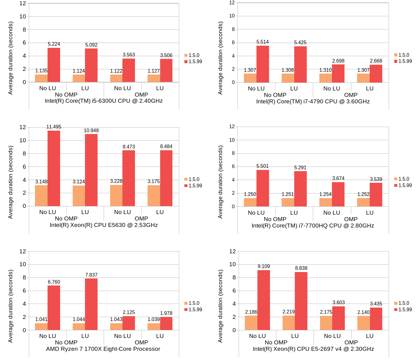
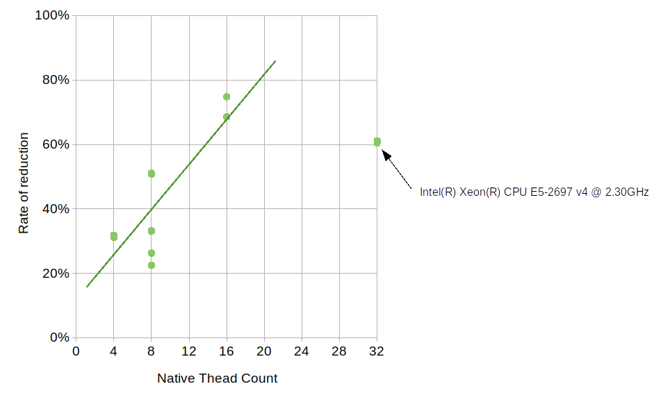
Here, LU and OMP stand for loop unrolling and OpenMP, respectively. The results from each machine consist of four groups each having two timing values, one with 1.5.0 and one with 1.5.99. Since 1.5.0 does not use neither loop unrolling nor OpenMP, its results show no variance between the groups, which is expected. The numbers for 1.5.99 are generally much higher than those of 1.5.0, but the use of OpenMP brings the numbers down considerably. Although how much OpenMP reduced the average duration varies from machine to machine, the number of available native threads likely plays some role. The reduction by OpenMP on Core i5 6300U (which comes with 4 native threads) is approximately 30%, the number on Ryzen 7 1700X (with 16 native threads) is about 70%, and the number on Core i7 4790 (with 8 native threads) is about 50%. The relationship between the native thread count and the rate of reduction somewhat follows a linear trend, though the numbers on Xeon E5-2697 v4, which comes with 32 native threads, deviate from this trend.

The effect of loop unrolling, on the other hand, is visible only to a much lesser degree; in all but two cases it has resulted in a reduction of 1 to 7 percent. The only exceptions are the Ryzen 7 without OpenMP which denoted an increase of nearly 16%, and the Xeon E5630 with OpenMP which denoted a slight increase of 0.1%.

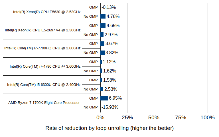
The 16% increase with the Ryzen 7 environment may well be an outlier, since the other test in the same environment (with OpenMP enabled) did result in a reduction of 7% – the highest of all tested groups.

Interpreting the results

Hopefully the results presented in this post are interesting and provide insight into the nature of the change in multi_type_vector in the upcoming 1.6.0 release. But what does this all mean, especially in the context of LibreOffice Calc? These are my personal thoughts.

  • From my own observation of having seen numerous bug reports and/or performance issues from various users of Calc, I can confidently say that the vast majority of cases involve reading and updating cell values without shifting of cells, either during file load, or during executions of features that involve massive amounts of cell I/O’s. Since those cases are primarily bottlenecked by block position search, the new implementation will bring a massive win especially in places where use of position hints was not practical. That being said, the performance of block search will likely see no noticeable improvements even after switching to the new implementation when the code already uses position hints with the old implementation.
  • While the increased overhead in block shifting, which is associated with insertion or deletion of rows in Calc, is a certainly a concern, it may not be a huge issue in day-to-day usage of Calc. It is worth pointing out that that what the benchmark measures is repeated insertions and shifting of highly fragmented blocks, which translates to repeated insertions or deletions of rows in Calc document where the column values consist of uniformly altering types. In normal Calc usage, it is more likely that the user would insert or delete rows as one discrete operation, rather than a series of thousands of repeated row insertions or deletions. I am highly optimistic that Calc can absorb this extra overhead without its users noticing.
  • Even if Calc encounters a very unlikely situation where this increased overhead becomes visible at the UI level, enabling OpenMP, assuming that’s practical, would help lessen the impact of this overhead. The benefit of OpenMP becomes more elevated as the number of native CPU threads becomes higher.

What’s next?

I may invest some time looking into potential use of GPU offloading to see if that would further speed up the block position update operations. The benefit of loop unrolling was not as great as I had hoped, but this may be highly CPU and compiler dependent. I will likely continue to dig deeper into this and keep on experimenting.

OpenCL test documents for Calc

opencl-doc-shot

Some of you have asked me previously whether or not we can share any test documents to demonstrate Calc’s new OpenCL-based formula engine. Thanks to AMD, we can now make available 3 test documents that showcase the performance of the new engine, and how it compares to Calc’s existing engine as well as Excel’s.

Download Platform
OpenCL-test-documents-Excel-64-bit.zip Excel (64-bit)
OpenCL-test-documents.zip Calc (Windows, 32-bit)
Calc (Linux, 32-bit)
Calc (Linux, 64-bit)
Excel (32-bit)

These files are intentionally in Excel format so that they can be used both in Calc and Excel. They also contain VBA script to automate the execution of formula cell recalculation and measure the recalculation time with a single button click.

All you have to do is to open one of these files, click “Recalculate” and wait for it to finish. It should give you the number that represents the duration of the recalculation in milliseconds.

Note that the 64-bit version of Excel requires different VBA syntax for calling native function in DLL, which is why we have a separate set of documents just for that version. You should not use these documents unless you want to test them specifically in the 64-bit version of Excel. Use the other one for all the rest.

On Linux, you need to use a reasonably recent build from the master branch in order for the VBA macro to be able to call the native DLL function. If you decide to run them on Linux, make sure your build is recent enough to contain this commit.

Once again, huge thanks to AMD for allowing us to share these documents with everyone!

Update on border lines

Just a quick update to my last post on getting Calc’s border line situation sorted out.

As of last post, the border lines were pretty in good shape as far as printing to paper, but it was still less than satisfactory when rendered on screen. Lines looked generally fatter and the dashes line were unevenly positioned. I had some ideas that I wanted to try out in order to make the border lines look prettier on screen. So I went ahead and spent a few extra days to give that a try, and I’m happy to report that that effort paid off.

To recap, this is what the border lines looked like as of last Friday.

screen-calc-after

and this is what they look like now:

screen-calc-followup

The lines are skinnier, which in my opinion make them look slicker, and the dashes lines are now evenly spaced and look much better.

The art of drawing border lines

I spent this past week on investigating a collection of various problems surrounding how Calc draws cell borders. The problem is very hard to define and can become very subjective depending on who you talk to. Having said that, if you ever imported an Excel document that makes elaborate use of cell borders into Calc, you may often have seen that the borders were printed somewhat differently than what you would have expected.

Here is an example. This is a very small test Excel document that I made that contains all cell border types that Excel supports. When you open this document in Excel and print it on paper, here is what you get.

excel-print

When you open this document in Calc and print it, you probably get something like this:

calc-print-before

You’ll immediately notice that some of the lines (hair, dashed and double lines to be precise) are not printed at all! Not only that, thin, medium and thick lines are a little skinner than those of Excel’s, the dotted line is barely visible, the medium dashed line looks a lot different, and the rest of the dashed lines all became solid lines.

Therefore, it was time for action.

Results

I’ll spare you the details, but the good news is that after spending a week in various parts of the code base, I’ve been able to fix most of the major issues. Here is what Calc prints now using the build from the latest master branch:

calc-print-after

There are still some minor discrepancies from Excel’s borders, such as the double line being a bit too thinner, the dotted line being not as dense as Excel’s etc. But I consider this a step in the right direction. The dashed and medium dashed lines look much better to my eye, and the thicknesses of these lines are more comparable to Excel’s.

The dash-dot and dash-dot-dot lines still become solid lines since we don’t yet support those line types, but that can be worked on at a later time.

So, this is all good, right?

Not quite. One of the reasons why the cell borders became such a big issue was that we previously focused too much on getting them to display correctly on screen. Unfortunately, the resolution of a typical PC monitor is not high enough to accurately depict the content of your document, so what you see on screen is a pixelized approximation of the actual content. When printing to a paper, on the other hand, the content gets depicted much more accurately simply because you get much higher resolution when printing.

I’ll give you a side-by-side comparison of how the content of the same document gets displayed in Excel (2010), Calc 4.2 (before my change), and Calc master (with my change) all at 100% zoom level.

First up is Excel:

screen-excel

The lines all look correct, unsurprisingly. One thing to note is that when displaying Excel approximates a hairline with a very thin, densely dotted line to differentiate it from a thin line both of which are one pixel high. But make no mistake; hairline by definition is a solid line. This is just a trick Excel employs in order to make the hairline look thinner than the thin line counterpart.

Then comes Calc as of 4.2 (before my change):

screen-calc-before

The hairline became a finely-dashed line both on display and in internal representation. Aside from that, both dashed and medium dashed lines look a bit too far apart. Also, the double line looks very much single. In terms of the line thicknesses, however, they do look very much comparable to Excel’s. Let me also remind you that Excel’s dash-dot and dash-dot-dot lines currently become solid lines in Calc because we don’t support these line types yet.

Now here is what Calc displays after my change:

screen-calc-after

The hair line is a solid line since we don’t use the same hair line trick that Excel uses. The dotted and dashes lines look much denser and in my opinion look better. The double line is now really double. The line thicknesses, however, are a bit off even though they are internally more comparable to Excel’s (as you saw in the printout above). This is due to the loss of precision during rasterization of the border lines, and for some reason they get fatter. We previosly tried to “fix” this by making the lines thinner internally, but that was a wrong approach since that also made the lines thinner even when printed, which was not a good thing. So, for now, this is a compromise we’ll have to live with.

But is there really nothing we can do about this? Well, we could try to apply some correction to make the lines look thinner on screen, and on screen only. I have some ideas how we may be able to achieve that, and I might give that a try during my next visit.

That, and we should also support those missing dash-dot, and dash-dot-dot line types at some point.

Speedier export of rich text cells

Here is another performance improvement that just landed on master.

Background

It was brought to our attention that the performance of saving documents to ODF spreadsheet format had been degrading quite noticeably. This was especially true when the document contained lots of what we call rich text cells. Rich text cells are those cells that contain text with mixed format spans, or text that consists of multiple lines. These cells are handled differently from simple strings internally, and have slightly more overhead than the simple string counterparts. Because of this, saving a document full of such texts was always slower than saving one with just numbers and simple strings.

However, even with this unavoidable overhead, the performance of saving rich text cells was clearly going in the wrong direction. Therefore it was time to act.

Long story short, after many days of code reading and writing, I brought it to a state where I can share some numbers.

Measuring export performance

I measured the performance of exporting rich text cells in the following steps.

  1. Create a new spreadsheet document.
  2. Type in cell A1 3 lines of ‘libreoffice’. Here, you can hit Ctrl-Enter to move to the next line within the same cell.
  3. Copy A1, select A1:N1000 and paste, to replicate the content of A1 to all cells in the range.
  4. Save the document as ODF spreadsheet document, and measure its duration.

Results

I performed the above measurement with 3.5, 3.6, 4.0, 4.1, and the latest master (slated to become 4.2) builds, and these are the numbers.
edit-text-export-ods-perf

It is clear from this chart that the performance started to suffer first in version 3.6, then gradually worsened over 4.0 and 4.1. The good news is that we have managed to bring the number back down in the master build, even lower than that of 3.5 which I used as the point of reference. Not just slightly lower, but much, much lower.

I don’t know about you, but I’m quite happy with this result.

Shared formula to reduce memory usage

This week I have finally finished implementing a true shared formula framework in Calc core which allows Calc to share token array instances between adjacent formula cells if they contain identical set of formula tokens. Since one of the major benefits of sharing formula token arrays is reduced memory footprint, I decided to measure the trend in Calc’s memory usages since 4.0 all the way up to the latest master, to see how much impact this shared formula work has made in Calc’s overall memory footprint.

Test document

Here is the test document I used to measure Calc’s memory usage

shared-formula-memory-test.ods

This ODF spreadsheet document contains 100000 rows of cells in 4 columns of which 399999 are formula cells. Column A contains a series of integers that grow linearly down the column. Here, only the first cell (A1) is a numeric cell while the rest are all formula cells that reference their respective immediate upper cell. Cells in Column B all reference their immediate left in Column A, cells in Column C all reference their immediate left in Column B, and so on. References used in this document are all relative references; no absolute references are used.

Tested builds

I’ve tested a total of 4 builds. One is the 4.0.1 build packaged for openSUSE 11.4 (x64) from the openSUSE repository, one is the 4.0.6 build built from the 4.0 branch, one is the 4.1.1 build built from the 4.1 branch, and the last one is the latest from the master branch. With the exception of the packaged 4.0.1 build, all builds are built locally on my machine running openSUSE 11.4 (x64). Also on the master build, I’ve tested memory usage both with and without shared formulas.

Results

In each tested build, the memory usage was measured by directly opening the test document from the command line and recording the virtual memory usage in GNOME system monitor. After the document was loaded, I allowed for the virtual memory reading to stabilize by waiting several seconds before recording the number. The results are presented graphically in the following chart.

shared-memory-graph

The following table shows the actual numbers recorded.

Build Virtual memory
4.0.1 (packaged by openSUSE) 4.0 GiB
4.0.6 892.1 MiB
4.1.1 858.4 MiB
master (no shared formula) 842.2 MiB
master (shared formula) 763.9 MiB

Additionally, I’ve also measured the number of token array instances between the two master builds (one with shared formula and one without), and the build without shared formula created 399999 token array instances (exactly 4 x 100000 – 1) upon file load, whereas the build with shared formula created only 4 token array instances. This likely accounts for the difference of 78.3 MiB in virtual memory usage between the two builds.

Effect of cell storage rework

One thing worth noting here is that, even without shared formulas, the numbers clearly show a steady decline of Calc’s memory usage from 4.0 to 4.1, and to the current master. While we can’t clearly infer from these numbers alone what caused the memory usage to shrink, I can say with reasonable confidence that the cell storage rework we did during the same period is a significant factor in such memory footprint shrinkage. I won’t go into the details of the cell storage rework here; I’ll reserve that topic for another blog post.

Oh by the way, I have absolutely no idea why the 4.0.1 build packaged from the openSUSE repository shows such high memory usage. To me this looks more like an anomaly, indicative of earlier memory leaks we had later fixed, different custom allocator that only the distro packaged version uses that favors large up-front memory allocation, or anything else I haven’t thought of. Either way, I’m not counting this as something that resulted from any of our improvements we did in Calc core.

SUSE Hack Week

Last week was SUSE’s Hack Week – an event my employer does periodically to allow us – hard working engineers – to go wild with our wildest ideas and execute them in one week. Just like what I did at my last Hack Week event, I decided to work on integration of Orcus library into LibreOffice once again, to pick up on what I’d left off from my previous integration work.

Integration bits

Prior to Hack Week, orcus was already partially integrated; it was used to provide the backend functionality for Calc’s XML Source feature, and experimental support for Gnumeric file import. The XML Source side was pretty well integrated, but the normal file import side was only partially integrated. Lots of essential pieces were still missing, the largest of which were

  • support for multiple filters from a single external filter provider source (such as orcus),
  • progress indicator in the status bar, and
  • proper type detection by analyzing file content rather than its extension (which we call “deep detection”).

In short, I was able to complete the first two pieces during Hack Week, while the last item still has yet to be worked on. Aside from this, there are still more minor pieces missing, but perhaps I can work on the remaining bits during the next Hack Week.

Enabling orcus in your build

If you have a recent enough build from the master branch of the LibreOffice repository, you can enable imports via orcus library by

  1. checking the Enable experimental features box in the Options dialog, and
  2. setting the environment variable LIBO_USE_ORCUS to YES before launching Calc.

This will overwrite the stock import filters for ODS, XLSX and CSV. At present, orcus only performs file extension based detection rather than content based one, so be mindful of this when you try this on your machine. To go back to the current import filters, simply disable experimental features, or unset the environment variable.

Note that I’ve added this bits to showcase a preview of what orcus can potentially do as a future import filter framework. As such, never use this in production if you want stable file loading experience, or don’t file bugs against this. We are not ready for that yet. Orcus filters are still missing lots and lots of features.

Also note that, while in theory you could enable orcus with the Windows build, the performance of orcus on Windows may not be that impressive; in fact, in some cases slower than the current filters. That is because orcus relies on strtod and strtol system calls to convert string numbers into numeric values, and their implementation depend on the platform. And the performance of MSVC’s strtod implementation is known to be suboptimal compared to those of gcc and clang on Linux. I’m very much aware of this, and will work on addressing this at a later time.

Performance comparison

This is perhaps the most interesting part. I wanted to do a quick performance comparison and see how this orcus filter stands up against the current filter. Given the orcus filter is still only capable of importing raw cell values and not any other features or properties (not even cell formats), I’ve used this test file which only consists of raw text and numeric values in a 8-by-300000 range, to measure the load times that are as fair and representative as I could make them. Here is the result on my machine running openSUSE 11.4:

xlsx-load-times

The current filter, which has undergone its set of performance optimizations on raw cell values, still spends upwards of 50 seconds. Given that it used to take minutes to load this file, it’s still an improvement.

The orcus filter, on the other hand, combined with the heavily optimized load handler in Calc core that I put in place during Hack Week, can load the same file in 4.5 seconds. I would say that is pretty impressive.

I also measured the load time on the same file using Excel 2007, on the same machine running on top of wine, and the result was 7.5 seconds. While running an Windows app via wine emulation layer may incur some performance cost, this page suggests that it should not be noticeable, if any. And my own experience of running various versions of Excel via wine backs up that argument. So this number should be fairly representative of Excel’s native performance on the same hardware.

Considering that my ultimate goal with orcus is to beat Excel on performance on loading its own files (or at least not be slower than Excel), I would say we are making good progress toward that goal.

That’s all for today. Thank you, ladies and gentlemen.

Orcus integration into LibreOffice

Last week was SUSE Hack Week, where we SUSE engineers were encouraged to be creative and work on whatever project that we had been dying to work on.

Given this opportunity, I decided to try integrating my orcus library project into LibreOffice proper to see how much improvement we could make in the performance of loading spreadsheet documents.

I’ll leave the detailed description and goal of orcus project for another blog post, but in short, orcus is an independent library designed to process spreadsheet documents, and is also designed to be useable from an application that would like to use it to load documents. It’s currently still work in progress, and is not even in alpha quality. So, I intentionally don’t release orcus library packages on an official basis.

Integration work

The main difficulty with integrating orcus into LibreOffice proper was dealing with the very intricate loading process that LibreOffice uses for all existing filters. It first goes through an elaborate type detection process, which loads the content of the file into memory in order for the type detection code to parse it. Once the correct type is determined, LibreOffice then instantiates correct frame loader and start the actual loading process. I’ve explained all of this in detail in this blog post of mine.

Orcus, on the other hand, only needs a file path, and it does the rest. And it pushes data to the call back functions provided by the client code as it parses the file. It was this difference in overall loading process that made the integration of orcus into LibreOffice all the more challenging. And even though the hack week itself lasted only one week, I had spent months prior to it just to study the type detection code and other auxiliary code that makes up the whole file loading process in order to come up with an elegant way to add hook for orcus.

Long story short, I was able to come up with a way to hook orcus such that LibreOffice relinquishes all its file loading to the orcus library, and only handles callbacks. To make this work, I first packaged orcus into an installable rpm package using the openSUSE build service, locally installed that package, then added –with-system-orcus configure option to allow LibreOffice to find the library. The entire change needed to add hook is condensed into this commit.

Using CSV filter as an experiment

As an initial experiment, I replaced the current csv import filter with one from orcus, just to see how this overall process works. The results are very encouraging.

With a very large csv file I created via this python script:

#!/usr/bin/env python
 
import sys
 
for i in xrange(0, 65536):
    for j in xrange(1, 101):
        val = i * 1.0 / j
        sys.stdout.write("%g,"%val)
    sys.stdout.write("end\n")

the current filter spends roughly 27 seconds to load this file, which is not too bad given the sheer size of the file (~50Mb). The orcus filter, on the other hand, spends only 11 seconds to load the same file.

However, the orcus filter code path still skips a number of steps that need to be performed if it were to be used in the production build, such as

  • drawing progress bar in the status bar area,
  • calculating row heights for rows that include multi-line cell contents, and
  • probably something else I forget to mention here.

Given some of these can be quite expensive, the above numbers may not be fully comparable. Despite that, these initial numbers show a great promise on the performance improvement that may result from using the orcus library.

Future work

First of all, we will not switch to the orcus csv filter anytime soon. Although I’d like to see that happen at some point in the future, there are still lots of missing pieces in the orcus csv filter that prevent us from using it in the production build. My plan with orcus is therefore limited to addition of new filters, and my immediate plan is to develop new XML import and export filters using orcus, and integrate it into LibreOffice. This should also provide a stepping stone for any additional filters that may come up later, as well as replacing some of the existing filters as the need arises.

That’s all for now. Thanks for reading!

mdds::multi_type_vector explained

As my previous post just mentioned, mdds 0.6.0 is finally released which contains two new data structures: multi_type_vector and multi_type_matrix. I’d like to explain a little more about multi_type_vector in this post because, of all the data structures I’ve added to mdds over the course of its project life, I firmly believe this structure deserves some explanation.

What motivated multi_type_vector

The initial idea for this structure came from a discussion I had with Michael Meeks over two years ago in Nuremberg, Germany. Back then, he was dumping his idea on me about how to optimize cell storage in LibreOffice Calc, and his idea was that, instead of storing cell values wrapped around cell objects allocated on the heap and storing them in a column array, we store raw cell values directly in an array without the cell object wrappers. This way, if you have a column filled with numbers from top down, those values are guaranteed to be placed in a contiguous region in memory space which is more likely to be in the same memory page unless their size exceeds the memory page size. By contrast, if you store cell values wrapped inside cell objects that are allocated on the heap, those values are most likely scattered all around the memory space and probably located in many different memory pages.

Now, one of the most common operations that typical spreadsheet users do is to operate on numbers in cells. It could be summing up their totals, calculating their average, determining their minimum and maximum values and so on and so forth. To make these operations happen, the program first needs to fetch all the cell values before it can work on them.

Assume that these values are stored inside cell objects which are located in hundreds of memory pages. The mere action of fetching the cell values alone requires loading all of these memory pages, which causes the CPU to fetch them from the main memory in order to access them. Worse, if some of those pages are located in instead of the physical memory space but in the virtual memory space, it causes page fault, which further degrades performance since that particular memory page must be swapped in from disk. In contrast, if they are all located in a single memory page (or just several of them instead of hundreds), it just needs to fetch just once or several times, depending on the size of the data being fetched.

Moreover, most CPUs these days come equipped with CPU caches to cache recently-fetched memory pages in order to speed up subsequent access to them. Because of this, keeping all your data in the same page reduces the chance of the CPU fetching it from the main memory (or the worse case from the virtual memory), which is slower than fetching it from the caches.

Let’s visualize this idea for a moment. The current cell storage looks like this:

As you can see, cells are scattered in different pages. To access them all, you need to load all of these pages that contain the requested cell objects.

Compare that with the following illustration:

where all requested cell values are stored in a single array that’s located in a single page. I hope it’s obvious by now which one actually fetches data faster.

Calc currently employs the former storage model, and our hope is to make Calc’s storage model more efficient both space- and time-wise by switching to the latter model.

Applying this to the design

One difficulty with applying this concept to column storage is that, a column in a typical spreadsheet application allows you to store values of different types. Cells containing a bunch of test scores may have in the same column a title cell at the top that stores the text “Score”. Likewise, those test scores may be followed by an empty cell followed by a bunch of formula cells containing formula expressions summing, averaging, or counting the test scores. Since one array can only hold values of identical type, this requires us to use a separate array for each segment of identical cell type.

With that, the column storage structure becomes somewhat like this:

An empty cell segment doesn’t store any value array, but it does store its size which is necessary to calculate the logical position of the next non-empty element.

This is the basic design of the multi_type_vector structure. It stores values of each identical type in a single, secondary value array while the primary column array stores the memory locations of all secondary value arrays. It’s important to point out that, while I used the spreadsheet use case as an example to explain the basic idea of the structure, the structure itself can be used in other, much broader use cases, and is not specific to spreadsheet applications.

In the next section, I will talk about challenges I have faced while implementing this structure. But first one terminology note: from now on I will use the term “element block” (or simply “block”) to refer to what was referred to as “secondary value array” up to this point. I use this name in my implementation code too, so using this name makes easier for me to explain things.

The challenges

The basic design of multi_type_vector is not that complicated and was not very challenging to understand and implement. What was more challenging was to handle cases where a value, or a series of values, are inserted over a block or blocks of different types. There are a variety of ways to insert new values into this container, and sometimes the new values overlap the existing blocks of different types, or overlap a part of an existing block of the same type and a part of a block of a different type, and so on and so forth. Because the basic design of the container requires that the type of every element block differs from its neighbors’, some data insertions may cause the container to need to re-organize its element block structure. This posed quite a challenge since multi_type_vector supports the following methods of modifications:

  • set a single value to overwrite an existing one if any (set() method, 2-parameter variant),
  • set a sequence of values to overwrite existing values if any (set() method, 3-parameter variant),
  • insert a sequence of values and shift those existing values that occur below the insertion position (insert() method),
  • set a segment of existing values empty (set_empty() method), and
  • insert a sequence of empty values and shift those existing value that occur below the insertion position (insert_empty() method),

and each of these scenarios requires different strategy for element block re-organization. Non-overwriting data insertion scenarios (insert() and insert_empty()) were somewhat easier to handle than the overwriting data insertion scenarios (set() and set_empty()), as the latter required more branching and significantly more code to cover all cases.

This challenge was further exacerbated by additional requirement to support a “managed” element block that stores pointers to objects whose life cycle is managed by the block. I decided to add this one for convenience reasons, to allow transitioning the current cell storage model into the new storage model in several phases rather than doing it in one big-bang change. During the transition phase, we will likely convert the number and string cells into raw value element blocks, while keeping more complex cell structures such as formula cells still wrapped in their current form. This means that, during the transition we will have element blocks storing pointers to heap-allocated formula cell objects scattered across memory space. Eventually these formula objects need to be stored in a contiguous memory space but that will have to wait after the transition phase.

Supported data types

Template containers are supposed to work with any custom types, and multi_type_vector is no exception. But unlike most standard template containers which normally have one primary data type (and perhaps another one for associative containers), multi_type_vector allows storage of unspecified numbers of data types.

By default, multi_type_vector supports the following data types: bool, short, unsigned short, int, unsigned int, long, unsigned long, double, and std::string. If these data types are all you need when using multi_type_vector, then you won’t have to do anything extra, and just instantiate the template instance by

typedef mdds::multi_type_vector<mdds::mtv::element_block_func> mtv_type;

and start using it like so:

mtv_type data(10); // set initial size to 10.
 
// insert values.
data.set(0, 1.1);
data.set(1, true);
data.set(3, std::string("Foo"));
...

But if you need to store other types of data, you’ll need to do a little more work. Let’s say you have this class type:

class my_custom_foo
{
    ....
};

and you want to store instances of this class in multi_type_vector. I’ll skip the actual definition of this class, but let’s assume that the basic stuff such as default and copy constructors, equality operator etc are all implemented and working properly.

First, you need to define a unique numeric ID for your custom type. Each element type must be associated with a numeric ID. The IDs for standard data types are defined as follows:

namespace mdds { namespace mtv {
 
typedef int element_t;
 
const element_t element_type_empty = -1;
 
const element_t element_type_numeric = 0;
const element_t element_type_string  = 1;
const element_t element_type_short   = 2;
const element_t element_type_ushort  = 3;
const element_t element_type_int     = 4;
const element_t element_type_uint    = 5;
const element_t element_type_long    = 6;
const element_t element_type_ulong   = 7;
const element_t element_type_boolean = 8;
 
}}

These values are what gets returned by calling the get_type() method. When you are adding a new data type, you’ll need to add a new ID for it. Here is how to do it the safe way:

const mdds::mtv::element_t element_my_custom_type = mdds::mtv::element_type_user_start;

The value of element_type_user_start defines the starting number of all custom type IDs. IDs for the standard types all come before this value. If you only want to define one custom type ID, then just using that value will be sufficient. If you need another ID, just add 1 to it and use it for that type. As long as each ID is unique, it doesn’t really matter what their actual values are.

Next, you need to choose the block type. There are 3 block types to choose from:

  • mdds::mtv::default_element_block
  • mdds::mtv::managed_element_block
  • mdds::mtv::noncopyable_managed_element_block

The last 2 are relevant only when you need a managing pointer element block to store heap objects. Right now, let’s just use the default element block for your custom type.

typedef mdds::mtv::default_element_block<element_my_custom_type, my_custom_foo> my_custom_element_block;

With this, define all necessary callback functions for this custom type via following pre-processor macro:

MDDS_MTV_DEFINE_ELEMENT_CALLBACKS(my_custom_foo, element_my_custom_type, my_custom_foo(), my_custom_element_block)

Note that these callbacks functions are called from within multi_type_vector via unqualified call, so it’s essential that they are in the same namespace as the custom data type in order to satisfy C++’s argument-dependent lookup rule.

So far so good. The last step that you need to do is to define a structure of element block functions. This is also a boiler plate, and for a single custom type case, you can define something like this:

struct my_element_block_func
{
    static mdds::mtv::base_element_block* create_new_block(
        mdds::mtv::element_t type, size_t init_size)
    {
        switch (type)
        {
            case element_my_custom_type:
                return my_custom_element_block::create_block(init_size);
            default:
                return mdds::mtv::element_block_func::create_new_block(type, init_size);
        }
    }
 
    static mdds::mtv::base_element_block* clone_block(const mdds::mtv::base_element_block& block)
    {
        switch (mdds::mtv::get_block_type(block))
        {
            case element_my_custom_type:
                return my_custom_element_block::clone_block(block);
            default:
                return mdds::mtv::element_block_func::clone_block(block);
        }
    }
 
    static void delete_block(mdds::mtv::base_element_block* p)
    {
        if (!p)
            return;
 
        switch (mdds::mtv::get_block_type(*p))
        {
            case element_my_custom_type:
                my_custom_element_block::delete_block(p);
            break;
            default:
                mdds::mtv::element_block_func::delete_block(p);
        }
    }
 
    static void resize_block(mdds::mtv::base_element_block& block, size_t new_size)
    {
        switch (mdds::mtv::get_block_type(block))
        {
            case element_my_custom_type:
                my_custom_element_block::resize_block(block, new_size);
            break;
            default:
                mdds::mtv::element_block_func::resize_block(block, new_size);
        }
    }
 
    static void print_block(const mdds::mtv::base_element_block& block)
    {
        switch (mdds::mtv::get_block_type(block))
        {
            case element_my_custom_type:
                my_custom_element_block::print_block(block);
            break;
            default:
                mdds::mtv::element_block_func::print_block(block);
        }
    }
 
    static void erase(mdds::mtv::base_element_block& block, size_t pos)
    {
        switch (mdds::mtv::get_block_type(block))
        {
            case element_my_custom_type:
                my_custom_element_block::erase_block(block, pos);
            break;
            default:
                mdds::mtv::element_block_func::erase(block, pos);
        }
    }
 
    static void erase(mdds::mtv::base_element_block& block, size_t pos, size_t size)
    {
        switch (mdds::mtv::get_block_type(block))
        {
            case element_my_custom_type:
                my_custom_element_block::erase_block(block, pos, size);
            break;
            default:
                mdds::mtv::element_block_func::erase(block, pos, size);
        }
    }
 
    static void append_values_from_block(
        mdds::mtv::base_element_block& dest, const mdds::mtv::base_element_block& src)
    {
        switch (mdds::mtv::get_block_type(dest))
        {
            case element_my_custom_type:
                my_custom_element_block::append_values_from_block(dest, src);
            break;
            default:
                mdds::mtv::element_block_func::append_values_from_block(dest, src);
        }
    }
 
    static void append_values_from_block(
        mdds::mtv::base_element_block& dest, const mdds::mtv::base_element_block& src,
        size_t begin_pos, size_t len)
    {
        switch (mdds::mtv::get_block_type(dest))
        {
            case element_my_custom_type:
                my_custom_element_block::append_values_from_block(dest, src, begin_pos, len);
            break;
            default:
                mdds::mtv::element_block_func::append_values_from_block(dest, src, begin_pos, len);
        }
    }
 
    static void assign_values_from_block(
        mdds::mtv::base_element_block& dest, const mdds::mtv::base_element_block& src,
        size_t begin_pos, size_t len)
    {
        switch (mdds::mtv::get_block_type(dest))
        {
            case element_my_custom_type:
                my_custom_element_block::assign_values_from_block(dest, src, begin_pos, len);
            break;
            default:
                mdds::mtv::element_block_func::assign_values_from_block(dest, src, begin_pos, len);
        }
    }
 
    static bool equal_block(
        const mdds::mtv::base_element_block& left, const mdds::mtv::base_element_block& right)
    {
        if (mdds::mtv::get_block_type(left) == element_my_custom_type)
        {
            if (mdds::mtv::get_block_type(right) != element_my_custom_type)
                return false;
 
            return my_custom_element_block::get(left) == my_custom_element_block::get(right);
        }
        else if (mdds::mtv::get_block_type(right) == element_my_custom_type)
            return false;
 
        return mdds::mtv::element_block_func::equal_block(left, right);
    }
 
    static void overwrite_values(mdds::mtv::base_element_block& block, size_t pos, size_t len)
    {
        switch (mdds::mtv::get_block_type(block))
        {
            case element_my_custom_type:
                // Do nothing.  The client code manages the life cycle of these cells.
            break;
            default:
                mdds::mtv::element_block_func::overwrite_values(block, pos, len);
        }
    }
};

This is quite a bit of code, I know. I should definitely work on making it a bit simpler to use with a lot less typing in future versions of mdds. Anyway, with this in place, we can finally define the multi_type_vector type:

typedef mdds::multi_type_vector<my_element_block_func> my_mtv_type;

With all these bits in place, you can finally start using this container:

my_mtv_type data(10);
my_custom_foo foo;
data.set(0, foo);  // Insert a custom data element.
data.set(1, 12.3); // You can still use the standard data types.
...

That’s all I will talk about custom data types for now. I hope this gives you a glimpse of how this container works in general.

Future work

Since this is the very first incarnation of multi_type_vector, I have no doubt this still has a lot of issues to be worked out. One immediate issue that comes to mind is the performance of element position lookup. Given a logical position of the element, the container first has to locate the right element block that stores the specified element, but this lookup always happens from the first element block. So, if you are doing a continuous lookup of million’s of elements in a loop, the overall lookup speed can be quite slow since each lookup starts from the first block. Speeding up this operation is certainly a task to be worked on in the near future. Meanwhile, the user of this container can resort to using the iterators to iterate through the element blocks and their member elements.

Another issue is the verbosity of the element block function structure required for custom element blocks. This can be worked out by providing templatized structures per number of custom data types. This one is probably easier to solve, and I should look into that soon.

That’s all for now, ladies and gentlemen!

Performance improvement in opening ODS documents

I have great news to share with you. Calc’s ODS import filter in 3.5 should be substantially faster when you have documents with a large number of named ranges. Read on if you want to know more details.

What happened?

Laurent Godard, Markus Mohrhard, and myself have been working pretty hard in the past month to bring the performance of ODS import filter to a reasonable level, especially with documents containing a large number of named ranges.

Here is the background. Laurent uses LibreOffice as a platform for his professional extension, which makes heavy use of named ranges. It programmatically generates ODS documents and inserts hundred’s or thousand’s of named ranges as intermediary storage to further process the data. The problem was, however, our import performance with that kind of documents was so suboptimal that this process was taking a prohibitively long time. In order for his extension to perform optimally, our ODS import filter needed to be optimized, and optimized heavily.

During the Paris conference, we got our heads together in order to come up with a strategy to make that happen. Laurent was more than willing to participate this effort, and in the end, he did substantial amount of work profiling, analyzing code, coming up with optimization strategy and putting it altogether. Markus and I provided mentorship, code pointers, as well as occasional coding to accelerate this effort.

Our hope was to make it all happen in time for our first 3.5 release. And I’m very happy to say that we made it.

Benchmark

Since we are talking about performance, it won’t be complete without the actual numbers. So here goes.

Test document 1


Here is the first test document global500.ods. It contains 500 sheets, 12,500 global named ranges, and 12,500 formulas that reference them.

On my development machine, the last stable release 3.4.4 takes 14 seconds to open this document. While 14 seconds may not seem that slow, keep in mind that this machine is somewhat unfairly fast tailored for the abusive developer use, so the real world performance is likely much less impressive (you can probably multiply that number by 3 to get a rough idea of the real world performance). Anyhow, using the latest master branch on the same machine, this document opens roughly in 2 and a half seconds. That’s roughly 86% reduction in import time.

Test document 2


Here is the second, somewhat larger document global1000.ods. This document contains 1000 sheets, 25,000 named ranges and 25,000 formulas that reference them.

According to my benchmark performed in the same condition as the first document, 3.4.4 opens this document in 50 seconds, whereas in 3.5.0 it opens under 5 seconds. That’s about 90% reduction in import time. Pretty impressive!

Real power of open source

This story shows another aspect of this remarkable achievement worth mentioning. If you use an open source product such as LibreOffice in your business, and if it doesn’t perform the way you need it to, you can actually join the project as a developer and coordinate the effort with the upstream developers to make it happen. And depending on the nature of the change you want to see happen, it can happen very quickly as this story demonstrates.

I wanted to emphasize this because, while more and more businesses and institutions are embracing open source software, many of them tend to focus too much on the cost-saving aspect of it, thereby developing the wrong mindset that that’s what open source is all about. It isn’t. The real power of using open source software in your deployment is it gives you the ability to join and contribute to the project to influence the direction of its development. That gives you real flexibility in planning, and in my opinion the best way to harness the power of using open source software. The monetary cost-saving side of the benefit comes as a side effect but should be thought of only as an added bonus, not the primary reason for deploying open source software.