In my previous post, I explained the basic concept of multi_type_vector – one of the two new data structures added to mdds in the 0.6.0 release. In this post, I’d like to explain a bit more about multi_type_matrix – the other new structure added in the aforementioned release. It is also important to note that the addition of multi_type_matrix deprecates mixed_type_matrix, and is subject to deletion in future releases.
Basics
In short, multi_type_matrix is a matrix data structure designed to allow storage of four different element types: numeric value (double), boolean value (bool), empty value, and string value. The string value type can be either std::string, or one provided by the user. Internally, multi_type_matrix is just a wrapper to multi_type_vector, which does most of the hard work. All multi_type_matrix does is to translate logical element positions in 2-dimensional space into one-dimensional positions, and pass them onto the vector. Using multi_type_vector has many advantages over the previous matrix class mixed_type_matrix both in terms of ease of use and performance.
One benefit of using multi_type_vector as its backend storage is that, we will no longer have to differentiate densely-populated and sparsely-populated matrix density types. In mixed_type_matrix, the user would have to manually specify which backend type to use when creating an instance, and once created, it wasn’t possible to switch from one to the other unless you copy it wholesale. In multi_type_matrix, on the other hand, the user no longer has to specify the density type since the new storage is optimized for either density type.
Another benefit is the reduced storage cost and improved latency in memory access especially when accessing a sequence of element values at once. This is inherent in the use of multi_type_vector which I explained in detail in my previous post. I will expand on the storage cost of multi_type_matrix in the next section.
Storage cost
The new multi_type_matrix structure generally provides better storage efficiency in most average cases. I’ll illustrate this by using the two opposite extreme density cases.
First, let’s assume we have a 5-by-5 matrix that’s fully populated with numeric values. The following picture illustrates how the element values of such numeric matrix are stored.

In mixed_type_matrix with its filled-storage backend, the element values are either 1) stored in heap-allocated element objects and their pointers are stored in a separate array (middle right), or 2) stored directly in one-dimensional array (lower right). Those initialized with empty elements employ the first variant, whereas those initialized with zero elements employ the second variant. The rationale behind using these two different storage schemes was the assertion that, in a matrix initialized with empty elements, most elements likely remain empty throughout its life time whereas a matrix initialized with zero elements likely get numeric values assigned to most of the elements for subsequent computations.
Also, each element in mixed_type_matrix stores its type as an enum value. Let’s assume that the size of a pointer is 8 bytes (the world is moving toward 64-bit systems these days), that of a double is 8 bytes, and that of an enum is 4 bytes. The total storage cost of a 5-by-5 matrix will be 8 x 25 + (8 + 4) x 25 = 500 bytes for empty-initialized matrix, and (8 + 4) x 25 = 300 bytes for zero-initialized matrix.
In contrast, multi_type_matrix (upper right) stores the same data using a single array of double’s, whose memory address is stored in a separate block array. This block array also stores the type of each block (int) and its size (size_t). Since we only have one numeric block, it only stores one int value, one size_t value, and one pointer value for the whole block. With that, the total storage cost of a 5-by-5 matrix will be 8 x 25 + 4 + 8 + 8 = 220 bytes. Suffice it to say that it’s less than half the storage cost of empty-initialized mixed_type_matrix, and roughly 26% less than that of zero-initialized mixed_type_matrix.
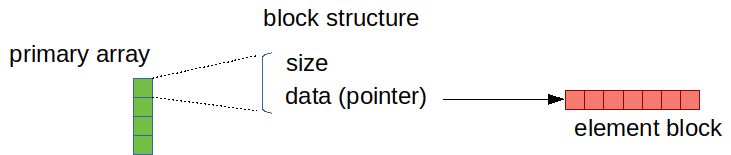
Now let’s a look at the other end of the density spectrum. Say, we have a very sparsely-populated 5-by-5 matrix, and only the top-left and bottom-right elements are non-empty like the following illustration shows:

In mixed_type_matrix with its sparse-storage backend (lower right), the element values are stored in heap-allocated element objects which are in turn stored in nested balanced-binary trees. The space requirement of the sparse-storage backend varies depending on how the elements are spread out, but in this particular example, it takes one 5-node tree, one 2-node tree, four single-node tree, and five element instances. Let’s assume that each node in each of these trees stores 3 pointers (pointer to left node, pointer right node and pointer to the value), which makes up 24 bytes of storage per node. Multiplying that by 11 makes 24 x 11 = 264 bytes of storage. With each element instance requiring 12 bytes of storage, the total storage cost comes to 24 x 11 + 12 x 6 = 336 bytes.
In multi_type_matrix (upper right), the primary array stores three element blocks each of which makes up 20 bytes of storage (one pointer, one size_t and one int). Combine that with one 2-element array (16 bytes) and one 4-element array (24 bytes), and the total storage comes to 20 x 3 + 8 * (2 + 4) = 108 bytes. This clearly shows that, even in this extremely sparse density case, multi_type_matrix provides better storage efficiency than mixed_type_matrix.
I hope these two examples are evidence enough that multi_type_matrix provides reasonable efficiency in either densely populated or sparsely populated matrices. The fact that one storage can handle either extreme also gives us more flexibility in that, even when a matrix object starts out sparsely populated then later becomes completely filled, there is no need to manually switch the storage structure as was necessary with mixed_type_matrix.
Run-time performance
Better storage efficiency with multi_type_matrix over mixed_type_matrix is one thing, but what’s equally important is how well it performs run-time. Unfortunately, the actual run-time performance largely depends on how it is used, and while it should provide good overall performance if used in ways that take advantage of its structure, it may perform poorly if used incorrectly.
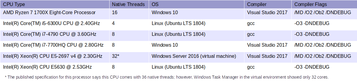
In this section, I will provide performance comparisons between multi_type_matrix and mixed_type_matrix in several difference scenarios, with the actual source code used to measure their performance. All performance comparisons are done in terms of total elapsed time in seconds required to perform each task. All elapsed times were measured in CPU time, and all benchmark codes were compiled on openSUSE 12.1 64-bit using gcc 4.6.2 with -Os compiler flag.
For the sake of brevity and consistency, the following typedef’s are used throughout the performance test code.
typedef mdds::mixed_type_matrix<std::string, bool>            mixed_mx_type;
typedef mdds::multi_type_matrix<mdds::mtm::std_string_trait> multi_mx_type; |
typedef mdds::mixed_type_matrix<std::string, bool> mixed_mx_type;
typedef mdds::multi_type_matrix<mdds::mtm::std_string_trait> multi_mx_type;
Instantiation
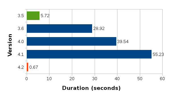
The first scenario is the instantiation of matrix objects. In this test, six matrix object instantiation scenarios are measured. In each scenario, a matrix object of 20000 rows by 8000 columns is instantiated, and the time it takes for the object to get fully instantiated is measured.
The first three scenarios instantiate matrix object with zero element values. The first scenario instantiates mixed_type_matrix with filled storage backend, with all elements initialized to zero.
mixed_mx_type mx(20000, 8000, mdds::matrix_density_filled_zero); |
mixed_mx_type mx(20000, 8000, mdds::matrix_density_filled_zero);
Internally, this allocates a one-dimensional array and fill it with zero element instances.
The second case is just like the first one, the only difference being that it uses sparse storage backend.
mixed_mx_type mx(20000, 8000, mdds::matrix_density_sparse_zero); |
mixed_mx_type mx(20000, 8000, mdds::matrix_density_sparse_zero);
With the sparse storage backend, all this does is to allocate just one element instance to use it as zero, and set the internal size value to specified size. No allocation for the storage of any other elements occur at this point. Thus, instantiating a mixed_type_matrix with sparse storage is a fairly cheap, constant-time process.
The third scenario instantiates multi_type_matrix with all elements initialized to zero.
multi_mx_type mx(20000, 8000, 0.0); |
multi_mx_type mx(20000, 8000, 0.0);
This internally allocates one numerical block containing one dimensional array of length 20000 x 8000 = 160 million, and fill it with 0.0 values. This process is very similar to that of the first scenario except that, unlike the first one, the array stores the element values only, without the extra individual element types.
The next three scenarios instantiate matrix object with all empty elements. Other than that, they are identical to the first three.
The first scenario is mixed_type_matrix with filled storage.
mixed_mx_type mx(20000, 8000, mdds::matrix_density_filled_empty); |
mixed_mx_type mx(20000, 8000, mdds::matrix_density_filled_empty);
Unlike the zero element counterpart, this version allocates one empty element instance and one dimensional array that stores all identical pointer values pointing to the empty element instance.
The second one is mixed_type_matrix with sparse storage.
mixed_mx_type mx(20000, 8000, mdds::matrix_density_sparse_empty); |
mixed_mx_type mx(20000, 8000, mdds::matrix_density_sparse_empty);
And the third one is multi_type_matrix initialized with all empty elements.
multi_mx_type mx(20000, 8000); |
multi_mx_type mx(20000, 8000);
This is also very similar to the initialization with all zero elements, except that it creates one empty element block which doesn’t have memory allocated for data array. As such, this process is cheaper than the zero element counterpart because of the absence of the overhead associated with creating an extra data array.
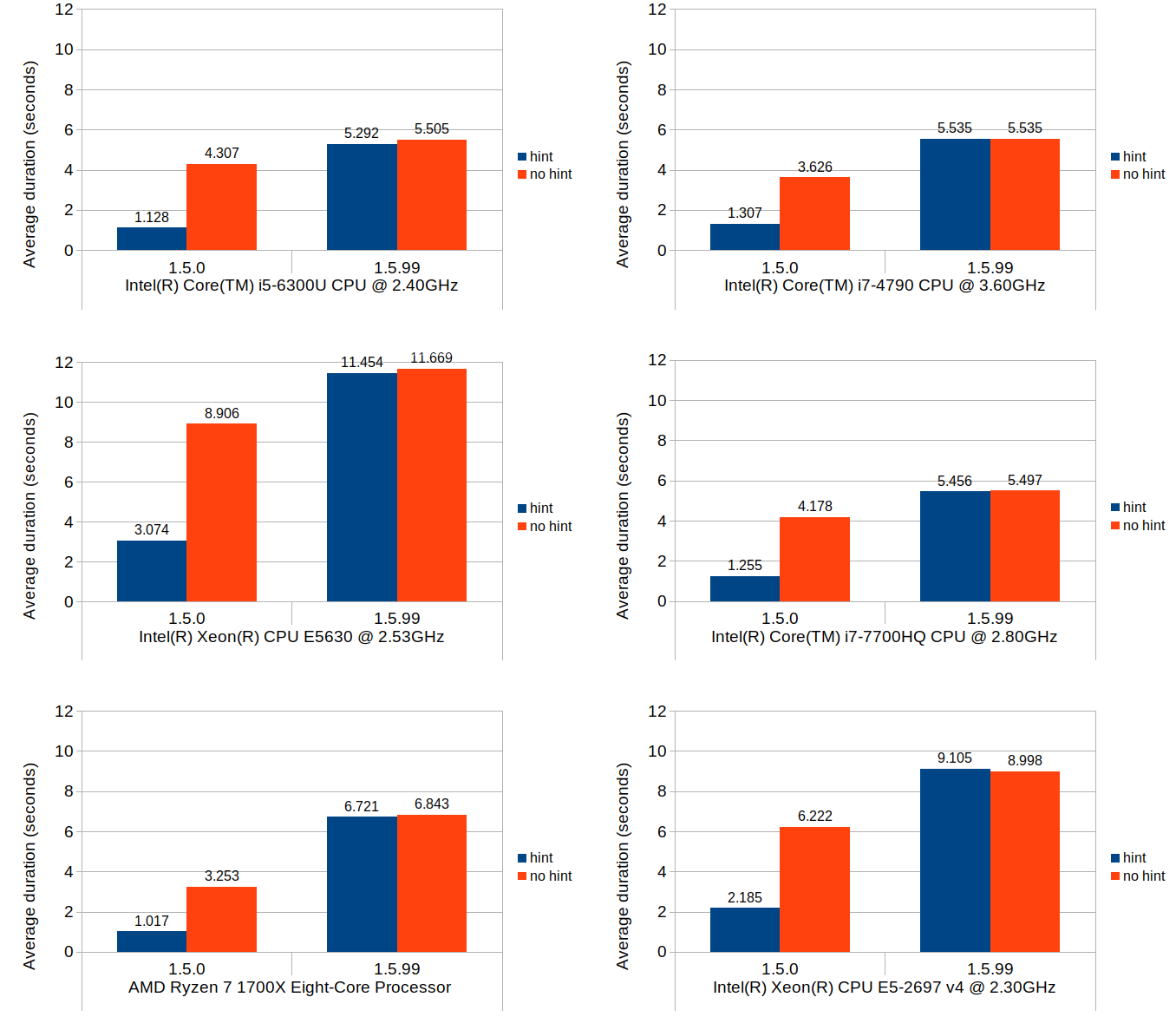
Here are the results:

The most expensive one turns out to be the zero-initialized mixed_type_matrix, which allocates array with 160 million zero element objects upon construction. What follows is a tie between the empty-initialized mixed_type_matrix and the zero-initialized multi_type_matrix. Both structures allocate array with 160 million primitive values (one with pointer values and one with double values). The sparse mixed_type_matrix ones are very cheap to instantiate since all they need is to set their internal size without additional storage allocation. The empty multi_type_matrix is also cheap for the same reason. The last three types can be instantiated at constant time regardless of the logical size of the matrix.
Assigning values to elements
The next test is assigning numeric values to elements inside matrix. For the remainder of the tests, I will only measure the zero-initialized mixed_type_matrix since the empty-initialized one is not optimized to be filled with a large number of non-empty elements.
We measure six different scenarios in this test. One is for mixed_type_matrix, and the rest are all for multi_type_matrix, as multi_type_matrix supports several different ways to assign values. In contrast, mixed_type_matrix only supports one way to assign values.
The first scenario involves assigning values to elements in mixed_type_matrix. Values are assigned individually inside nested for loops.
size_t row_size = 10000, col_size = 1000;

mixed_mx_type mx(row_size, col_size, mdds::matrix_density_filled_zero);

double val = 0.0;
for (size_t row = 0; row < row_size; ++row)
{
    for (size_t col = 0; col < col_size; ++col)
    {
        mx.set(row, col, val);
        val += 0.00001; // different value for each element
    }
} |
size_t row_size = 10000, col_size = 1000;
mixed_mx_type mx(row_size, col_size, mdds::matrix_density_filled_zero);
double val = 0.0;
for (size_t row = 0; row < row_size; ++row)
{
for (size_t col = 0; col < col_size; ++col)
{
mx.set(row, col, val);
val += 0.00001; // different value for each element
}
}
The second scenario is almost identical to the first one, except that it’s multi_type_matrix initialized with empty elements.
size_t row_size = 10000, col_size = 1000;

multi_mx_type mx(row_size, col_size);

double val = 0.0;
for (size_t row = 0; row < row_size; ++row)
{
    for (size_t col = 0; col < col_size; ++col)
    {
        mx.set(row, col, val);
        val += 0.00001; // different value for each element
    }
} |
size_t row_size = 10000, col_size = 1000;
multi_mx_type mx(row_size, col_size);
double val = 0.0;
for (size_t row = 0; row < row_size; ++row)
{
for (size_t col = 0; col < col_size; ++col)
{
mx.set(row, col, val);
val += 0.00001; // different value for each element
}
}
Because the matrix is initialized with just one empty block with no data array allocated, the very first value assignment allocates the data array just for one element, then all the subsequent assignments keep resizing the data array by one element at a time. Therefore, each value assignment runs the risk of the data array getting reallocated as it internally relies on std::vector’s capacity growth policy which in most STL implementations consists of doubling it on every reallocation.
The third scenario is identical to the previous one. The only difference is that the matrix is initialized with zero elements.
size_t row_size = 10000, col_size = 1000;

multi_mx_type mx(row_size, col_size, 0.0);

double val = 0.0;
for (size_t row = 0; row < row_size; ++row)
{
    for (size_t col = 0; col < col_size; ++col)
    {
        mx.set(row, col, val);
        val += 0.00001; // different value for each element
    }
} |
size_t row_size = 10000, col_size = 1000;
multi_mx_type mx(row_size, col_size, 0.0);
double val = 0.0;
for (size_t row = 0; row < row_size; ++row)
{
for (size_t col = 0; col < col_size; ++col)
{
mx.set(row, col, val);
val += 0.00001; // different value for each element
}
}
But this seemingly subtle difference makes a huge difference. Because the matrix is already initialized with a data array to the full matrix size, none of the subsequent assignments reallocate the array. This cuts the repetitive reallocation overhead significantly.
The next case involves multi_type_matrix initialized with empty elements. The values are first stored into an extra array first, then the whole array gets assigned to the matrix in one call.
size_t row_size = 10000, col_size = 1000;

multi_mx_type mx(row_size, col_size);

// Prepare a value array first.
std::vector<double> vals;
vals.reserve(row_size*col_size);
double val = 0.0;
for (size_t row = 0; row < row_size; ++row)
{
    for (size_t col = 0; col < col_size; ++col)
    {
        vals.push_back(val);
        val += 0.00001;
    }
}

// Assign the whole element values in one step.
mx.set(0, 0, vals.begin(), vals.end()); |
size_t row_size = 10000, col_size = 1000;
multi_mx_type mx(row_size, col_size);
// Prepare a value array first.
std::vector<double> vals;
vals.reserve(row_size*col_size);
double val = 0.0;
for (size_t row = 0; row < row_size; ++row)
{
for (size_t col = 0; col < col_size; ++col)
{
vals.push_back(val);
val += 0.00001;
}
}
// Assign the whole element values in one step.
mx.set(0, 0, vals.begin(), vals.end());
Operation like this is something that mixed_type_matrix doesn’t support. What the set() method on the last line does is to assign the values to all elements in the matrix in one single call; it starts from the top-left (0,0) element position and keeps wrapping values into the subsequent columns until it reaches the last element in the last column.
Generally speaking, with multi_type_matrix, assigning a large number of values in this fashion is significantly faster than assigning them individually, and even with the overhead of the initial data array creation, it is normally faster than individual value assignments. In this test, we measure the time it takes to set values with and without the initial data array creation.
The last scenario is identical to the previous one, but the only difference is the initial element values being zero instead of being empty.
size_t row_size = 10000, col_size = 1000;

multi_mx_type mx(row_size, col_size, 0.0);

// Prepare a value array first.
std::vector<double> vals;
vals.reserve(row_size*col_size);
double val = 0.0;
for (size_t row = 0; row < row_size; ++row)
{
    for (size_t col = 0; col < col_size; ++col)
    {
        vals.push_back(val);
        val += 0.00001;
    }
}

// Assign the whole element values in one step.
mx.set(0, 0, vals.begin(), vals.end()); |
size_t row_size = 10000, col_size = 1000;
multi_mx_type mx(row_size, col_size, 0.0);
// Prepare a value array first.
std::vector<double> vals;
vals.reserve(row_size*col_size);
double val = 0.0;
for (size_t row = 0; row < row_size; ++row)
{
for (size_t col = 0; col < col_size; ++col)
{
vals.push_back(val);
val += 0.00001;
}
}
// Assign the whole element values in one step.
mx.set(0, 0, vals.begin(), vals.end());
The only significant thing this code does differently from the last one is that it assigns values to an existing numeric data array whereas the code in the previous scenario allocates a new array before assigning values. In practice, this difference should not make any significant difference performance-wise.
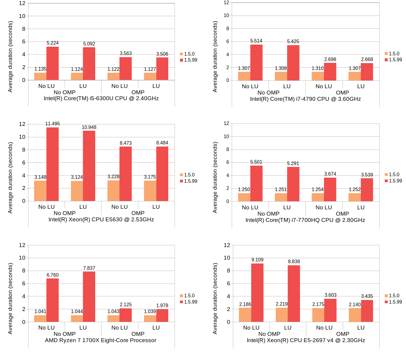
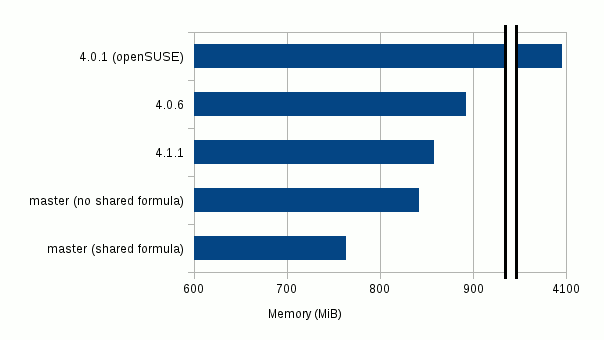
Now, let’s a take a look at the results.

The top orange bar is the only result from mixed_type_matrix, and the rest of the blue bars are from multi_type_matrix, using different assignment techniques.
The top three bars are the results from the individual value assignments inside loop (hence the label “loop”). The first thing that jumps out of this chart is that individually assigning values to empty-initialized multi_type_matrix is prohibitively expensive, thus such feat should be done with extra caution (if you really have to do it). When the matrix is initialized with zero elements, however, it does perform reasonably though it’s still slightly slower than the mixed_type_matrix case.
The bottom four bars are the results from the array assignments to multi_type_matrix, one initialized with empty elements and one initialized with zero elements, and one is with the initial data array creation and one without. The difference between the two initialization cases is very minor and well within the margin of being barely noticeable in real life.
Performance of an array assignment is roughly on par with that of mixed_type_matrix’s if you include the cost of the extra array creation. But if you take away that overhead, that is, if the data array is already present and doesn’t need to be created prior to the assignment, the array assignment becomes nearly 3 times faster than mixed_type_matrix’s individual value assignment.
Adding all numeric elements
The next benchmark test consists of fetching all numerical values from a matrix and adding them all together. This requires accessing the stored elements inside matrix after it has been fully populated.
With mixed_type_matrix, the following two ways of accessing element values are tested: 1) access via individual get_numeric() calls, and 2) access via const_iterator. With multi_type_matrix, the tested access methods are: 1) access via individual get_numeric() calls, and 2) access via walk() method which walks all element blocks sequentially and call back a caller-provided function object on each element block pass.
In each of the above testing scenarios, two different element distribution types are tested: one that consists of all numeric elements (homogeneous matrix), and one that consists of a mixture of numeric and empty elements (heterogeneous matrix). In the tests with heterogeneous matrices, one out of every three columns is set empty while the remainder of the columns are filled with numeric elements. The size of a matrix object is fixed to 10000 rows by 1000 columns in each tested scenario.
The first case involves populating a mixed_type_matrix instance with all numeric elements (homogenous matrix), then read all values to calculate their sum.
size_t row_size = 10000, col_size = 1000;

mixed_mx_type mx(row_size, col_size, mdds::matrix_density_filled_zero);

// Populate the matrix with all numeric values.
double val = 0.0;
for (size_t row = 0; row < row_size; ++row)
{
    for (size_t col = 0; col < col_size; ++col)
    {
        mx.set(row, col, val);
        val += 0.00001;
    }
}

// Sum all numeric values.
double sum = 0.0;
for (size_t row = 0; row < row_size; ++row)
    for (size_t col = 0; col < col_size; ++col)
sum += mx.get_numeric(row, col); |
size_t row_size = 10000, col_size = 1000;
mixed_mx_type mx(row_size, col_size, mdds::matrix_density_filled_zero);
// Populate the matrix with all numeric values.
double val = 0.0;
for (size_t row = 0; row < row_size; ++row)
{
for (size_t col = 0; col < col_size; ++col)
{
mx.set(row, col, val);
val += 0.00001;
}
}
// Sum all numeric values.
double sum = 0.0;
for (size_t row = 0; row < row_size; ++row)
for (size_t col = 0; col < col_size; ++col)
sum += mx.get_numeric(row, col);
The test only measures the second nested for loops where the values are read and added. The first block where the matrix is populated is excluded from the measurement.
In the heterogeneous matrix variant, only the first block is different:
// Populate the matrix with numeric and empty values.
double val = 0.0;
for (size_t row = 0; row < row_size; ++row)
{
    for (size_t col = 0; col < col_size; ++col)
    {
        if ((col % 3) == 0)
        {
            mx.set_empty(row, col);
        }
        else
        {
            mx.set(row, col, val);
            val += 0.00001;
        }
    }
} |
// Populate the matrix with numeric and empty values.
double val = 0.0;
for (size_t row = 0; row < row_size; ++row)
{
for (size_t col = 0; col < col_size; ++col)
{
if ((col % 3) == 0)
{
mx.set_empty(row, col);
}
else
{
mx.set(row, col, val);
val += 0.00001;
}
}
}
while the second block remains intact. Note that the get_numeric() method returns 0.0 when the element type is empty (this is true with both mixed_type_matrix and multi_type_matrix), so calling this method on empty elements has no effect on the total sum of all numeric values.
When measuring the performance of element access via iterator, the second block is replaced with the following code:
// Sum all numeric values via iterator.
double sum = 0.0;
mixed_mx_type::const_iterator it = mx.begin(), it_end = mx.end();
for (; it != it_end; ++it)
{
    if (it->m_type == mdds::element_numeric)
        sum += it->m_numeric;
} |
// Sum all numeric values via iterator.
double sum = 0.0;
mixed_mx_type::const_iterator it = mx.begin(), it_end = mx.end();
for (; it != it_end; ++it)
{
if (it->m_type == mdds::element_numeric)
sum += it->m_numeric;
}
Four separate tests are performed with multi_type_matrix. The first variant consists of a homogeneous matrix with all numeric values, where the element values are read and added via manual loop.
size_t row_size = 10000, col_size = 1000;

multi_mx_type mx(row_size, col_size, 0.0);

// Populate the matrix with all numeric values.
double val = 0.0;
for (size_t row = 0; row < row_size; ++row)
{
    for (size_t col = 0; col < col_size; ++col)
    {
        mx.set(row, col, val);
        val += 0.00001;
    }
}

// Sum all numeric values.
double sum = 0.0;
for (size_t row = 0; row < row_size; ++row)
    for (size_t col = 0; col < col_size; ++col)
sum += mx.get_numeric(row, col); |
size_t row_size = 10000, col_size = 1000;
multi_mx_type mx(row_size, col_size, 0.0);
// Populate the matrix with all numeric values.
double val = 0.0;
for (size_t row = 0; row < row_size; ++row)
{
for (size_t col = 0; col < col_size; ++col)
{
mx.set(row, col, val);
val += 0.00001;
}
}
// Sum all numeric values.
double sum = 0.0;
for (size_t row = 0; row < row_size; ++row)
for (size_t col = 0; col < col_size; ++col)
sum += mx.get_numeric(row, col);
This code is identical to the very first scenario with mixed_type_matrix, the only difference being that it uses multi_type_matrix initialized with zero elements.
In the heterogeneous matrix variant, the first block is replaced with the following:
multi_mx_type mx(row_size, col_size); // initialize with empty elements.
double val = 0.0;
vector<double> vals;
vals.reserve(row_size);
for (size_t col = 0; col < col_size; ++col)
{
    if ((col % 3) == 0)
        // Leave this column empty.
        continue;

    vals.clear();
    for (size_t row = 0; row < row_size; ++row)
    {
        vals.push_back(val);
        val += 0.00001;
    }

    mx.set(0, col, vals.begin(), vals.end());
} |
multi_mx_type mx(row_size, col_size); // initialize with empty elements.
double val = 0.0;
vector<double> vals;
vals.reserve(row_size);
for (size_t col = 0; col < col_size; ++col)
{
if ((col % 3) == 0)
// Leave this column empty.
continue;
vals.clear();
for (size_t row = 0; row < row_size; ++row)
{
vals.push_back(val);
val += 0.00001;
}
mx.set(0, col, vals.begin(), vals.end());
}
which essentially fills the matrix with numeric values except for every 3rd column being left empty. It’s important to note that, because heterogeneous multi_type_matrix instance consists of multiple element blocks, making every 3rd column empty creates roughly over 300 element blocks with matrix that consists of 1000 columns. This severely affects the performance of element block lookup especially for elements that are not positioned in the first few blocks.
The walk() method was added to multi_type_matrix precisely to alleviate this sort of poor lookup performance in such heavily partitioned matrices. This allows the caller to walk through all element blocks sequentially, thereby removing the need to restart the search in every element access. The last tested scenario measures the performance of this walk() method by replacing the second block with:
sum_all_values func;
mx.walk(func); |
sum_all_values func;
mx.walk(func);
where the sum_all_values function object is defined as:
class sum_all_values : public std::unary_function<multi_mx_type::element_block_node_type, void>
{
    double m_sum;
public:
    sum_all_values() : m_sum(0.0) {}

    void operator() (const multi_mx_type::element_block_node_type& blk)
    {
        if (!blk.data)
            // Skip the empty blocks.
            return;

        if (mdds::mtv::get_block_type(*blk.data) != mdds::mtv::element_type_numeric)
            // Block is not of numeric type.  Skip it.
            return;

        using mdds::mtv::numeric_element_block;
        // Access individual elements in this block, and add them up.
        numeric_element_block::const_iterator it = numeric_element_block::begin(*blk.data);
        numeric_element_block::const_iterator it_end = numeric_element_block::end(*blk.data);
        for (; it != it_end; ++it)
            m_sum += *it;
    }

    double get() const { return m_sum; }
}; |
class sum_all_values : public std::unary_function<multi_mx_type::element_block_node_type, void>
{
double m_sum;
public:
sum_all_values() : m_sum(0.0) {}
void operator() (const multi_mx_type::element_block_node_type& blk)
{
if (!blk.data)
// Skip the empty blocks.
return;
if (mdds::mtv::get_block_type(*blk.data) != mdds::mtv::element_type_numeric)
// Block is not of numeric type. Skip it.
return;
using mdds::mtv::numeric_element_block;
// Access individual elements in this block, and add them up.
numeric_element_block::const_iterator it = numeric_element_block::begin(*blk.data);
numeric_element_block::const_iterator it_end = numeric_element_block::end(*blk.data);
for (; it != it_end; ++it)
m_sum += *it;
}
double get() const { return m_sum; }
};
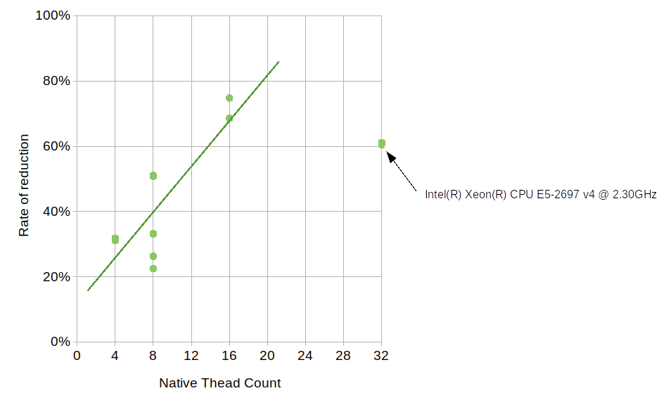
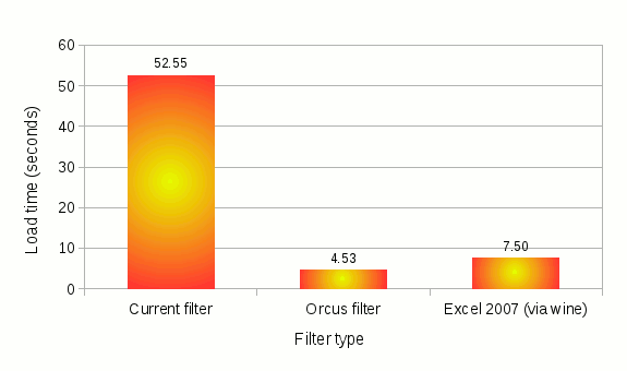
Without further ado, here are the results:

It is somewhat surprising that mixed_type_matrix shows poorer performance with iterator access as opposed to access via get_numeric(). There is no noticeable difference between the homogeneous and heterogeneous matrix scenarios with mixed_type_matrix, which makes sense given how mixed_type_matrix stores its element values.
On the multi_type_matrix front, element access via individual get_numeric() calls turns out to be very slow, which is expected. This poor performance is highly visible especially with heterogeneous matrix consisting of over 300 element blocks. Access via walk() method, on the other hand, shows much better performance, and is in fact the fastest amongst all tested scenarios. Access via walk() is faster with the heterogeneous matrix which is likely attributed to the fact that the empty element blocks are skipped which reduces the total number of element values to read.
Counting all numeric elements
In this test, we measure the time it takes to count the total number of numeric elements stored in a matrix. As with the previous test, we use both homogeneous and heterogeneous 10000 by 1000 matrix objects initialized in the same exact manner. In this test, however, we don’t measure the individual element access performance of multi_type_matrix since we all know by now that doing so would result in a very poor performance.
With mixed_type_matrix, we measure counting both via individual element access and via iterators. I will not show the code to initialize the element values here since that remains unchanged from the previous test. The code that does the counting is as follows:
// Count all numeric elements.
long count = 0;
for (size_t row = 0; row < row_size; ++row)
{
    for (size_t col = 0; col < col_size; ++col)
    {
        if (mx.get_type(row, col) == mdds::element_numeric)
            ++count;
    }
} |
// Count all numeric elements.
long count = 0;
for (size_t row = 0; row < row_size; ++row)
{
for (size_t col = 0; col < col_size; ++col)
{
if (mx.get_type(row, col) == mdds::element_numeric)
++count;
}
}
It is pretty straightforward and hopefully needs no explanation. Likewise, the code that does the counting via iterator is as follows:
// Count all numeric elements via iterator.
long count = 0;
mixed_mx_type::const_iterator it = mx.begin(), it_end = mx.end();
for (; it != it_end; ++it)
{
    if (it->m_type == mdds::element_numeric)
        ++count;
} |
// Count all numeric elements via iterator.
long count = 0;
mixed_mx_type::const_iterator it = mx.begin(), it_end = mx.end();
for (; it != it_end; ++it)
{
if (it->m_type == mdds::element_numeric)
++count;
}
Again a pretty straightforward code.
Now, testing this scenario with multi_type_matrix is interesting because it can take advantage of multi_type_matrix’s block-based element value storage. Because the elements are partitioned into multiple blocks, and each block stores its size separately from the data array, we can simply tally the sizes of all numeric element blocks to calculate its total number without even counting the actual individual elements stored in the blocks. And this algorithm scales with the number of element blocks, which is far fewer than the number of elements in most average use cases.
With that in mind, the code to count numeric elements becomes:
count_all_values func;
mx.walk(func); |
count_all_values func;
mx.walk(func);
where the count_all_values function object is defined as:
class count_all_values : public std::unary_function<multi_mx_type::element_block_node_type, void>
{
    long m_count;
public:
    count_all_values() : m_count(0) {}
    void operator() (const multi_mx_type::element_block_node_type& blk)
    {
        if (!blk.data)
            // Empty block.
            return;

        if (mdds::mtv::get_block_type(*blk.data) != mdds::mtv::element_type_numeric)
            // Block is not numeric.
            return;

        m_count += blk.size; // Just use the separate block size.
    }

    long get() const { return m_count; }
}; |
class count_all_values : public std::unary_function<multi_mx_type::element_block_node_type, void>
{
long m_count;
public:
count_all_values() : m_count(0) {}
void operator() (const multi_mx_type::element_block_node_type& blk)
{
if (!blk.data)
// Empty block.
return;
if (mdds::mtv::get_block_type(*blk.data) != mdds::mtv::element_type_numeric)
// Block is not numeric.
return;
m_count += blk.size; // Just use the separate block size.
}
long get() const { return m_count; }
};
With mixed_type_matrix, you are forced to parse all elements in order to count elements of a certain type regardless of which type of elements to count. This algorithm scales with the number of elements, much worse proposition than scaling with the number of element blocks.
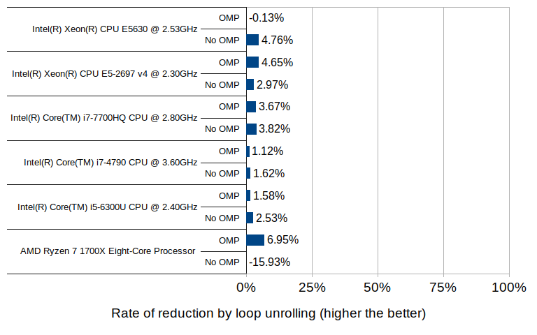
Now that the code has been presented, let move on to the results:

The performance of mixed_type_matrix, both manual loop and via iterator cases, is comparable to that of the previous test. What’s remarkable is the performance of multi_type_matrix via its walk() method; the numbers are so small that they don’t even register in the chart! As I mentions previously, the storage structure of multi_type_matrix replaces the problem of counting elements into a new problem of counting element blocks, thereby significantly reducing the scale factor with respect to the number of elements in most average use cases.
Initializing matrix with identical values
Here is another scenario where you can take advantage of multi_type_matrix over mixed_type_matrix. Say, you want to instantiate a new matrix and assign 12.3 to all of its elements. With mixed_type_matrix, the only way you can achieve that is to assign that value to each element in a loop after it’s been constructed. So you would write code like this:
size_t row_size = 10000, col_size = 2000;
mixed_mx_type mx(row_size, col_size, mdds::matrix_density_filled_zero);

for (size_t row = 0; row < row_size; ++row)
    for (size_t col = 0; col < col_size; ++col)
mx.set(row, col, 12.3); |
size_t row_size = 10000, col_size = 2000;
mixed_mx_type mx(row_size, col_size, mdds::matrix_density_filled_zero);
for (size_t row = 0; row < row_size; ++row)
for (size_t col = 0; col < col_size; ++col)
mx.set(row, col, 12.3);
With multi_type_matrix, you can achieve the same result by simply passing an initial value to the constructor, and that value gets assigned to all its elements upon construction. So, instead of assigning it to every element individually, you can simply write:
multi_mx_type(row_size, col_size, 12.3); |
multi_mx_type(row_size, col_size, 12.3);
Just for the sake of comparison, I’ll add two more cases for multi_type_matrix. The first one involves instantiation with a numeric block of zero’s, and individually assigning value to the elements afterward, like so:
multi_mx_type mx(row_size, col_size, 0.0);

for (size_t row = 0; row < row_size; ++row)
    for (size_t col = 0; col < col_size; ++col)
mx.set(row, col, 12.3); |
multi_mx_type mx(row_size, col_size, 0.0);
for (size_t row = 0; row < row_size; ++row)
for (size_t col = 0; col < col_size; ++col)
mx.set(row, col, 12.3);
which is algorithmically similar to the mixed_type_matrix case.
Now, the second one involves instantiation with a numeric block of zero’s, create an array with the same element count initialized with a desired initial value, then assign that to the matrix in one go.
multi_mx_type mx(row_size, col_size);

vector<double> vals(row_size*col_size, 12.3);
mx.set(0, 0, vals.begin(), vals.end()); |
multi_mx_type mx(row_size, col_size);
vector<double> vals(row_size*col_size, 12.3);
mx.set(0, 0, vals.begin(), vals.end());
The results are:

The performance of assigning initial value to individual elements is comparable between mixed_type_matrix and multi_type_matrix, though it is also the slowest of all. Creating an array of initial values and assigning it to the matrix takes less than half the time of individual assignment even with the overhead of creating the extra array upfront. Passing an initial value to the constructor is the fastest of all; it only takes roughly 1/8th of the time required for the individual assignment, and 1/3rd of the array assignment.
Conclusion
I hope I have presented enough evidence to convince you that multi_type_matrix offers overall better performance than mixed_type_matrix in a wide variety of use cases. Its structure is much simpler than that of mixed_type_matrix in that, it only uses one element storage backend as opposed to three in mixed_type_matrix. This greatly improves not only the cost of maintenance but also the predictability of the container behavior from the user’s point of view. That fact that you don’t have to clone matrix just to transfer it into another storage backend should make it a lot simpler to use this new matrix container.
Having said this, you should also be aware of the fact that, in order to take full advantage of multi_type_matrix to achieve good run-time performance, you need to
- try to limit single value assignments and prefer using value array assignment,
- construct matrix with proper initial value which also determines the type of initial element block, which in turn affects the performance of subsequent value assignments, and
- use the
walk() method when iterating through all elements in the matrix.
That’s all, ladies and gentlemen.